It never ceases to amaze me just how much is possible through the seemingly constrained model that DynamoDB gives us. It’s a fun puzzle to try to support access patterns beyond a simple key value lookup, or the retrieval of an ordered set of items.
The NoSQL gods teach us to store data in a way that mirrors our application’s functionality. This is often achieved by duplicating data so that it appears in multiple predefined sets for inexpensive retrieval.
This can get us a long way. However, it is common to delegate more complex queries to a secondary store, such as Elasticsearch or MySQL. DynamoDB remains the source of truth, but replicates to the secondary store via DynamoDB Streams and a Lambda function.
In many cases, a hybrid solution is the right approach, particularly when the model is complex and too challenging to fit into DynamoDB. Perhaps the scale DynamoDB provides simply isn’t needed for every single access pattern.
However, running two stores and replicating one into the other is definitely added complexity. Elasticsearch, even when used as a managed service, can still be a complex and expensive beast. What if it wasn’t needed? I believe it is desirable to keep things as lean as possible and only follow that path if it is necessary.
This series of posts explores what is possible with DynamoDB alone, starting naively, demonstrating problems and pitfalls along the way.
Part 1: Duplicating data with Lambda and DynamoDB streams to support filtering
Part 2: Using global secondary indexes and parallel queries to reduce storage footprint and write less code
Part 3: How to make pagination work when the output of multiple queries have been combined
Part 4: Storage and retrieval of comment statistics using index overloading and sparse indexes
Example scenario: a product comments system
We are tasked with producing a data model to store and retrieve the comments shown on each product page within an e-commerce site. A product has a unique identifier which is used to partition the comments. Each product has a set of comments. The most recent
20comments are shown beneath a product. Users can click a next button to paginate through older comments. As the front end system might be crawled by search engines, we do not want performance to degrade when older comments are requested.
This can be broken down into the following access patterns.
- AP1: Show all comments for a product, most recent first
- AP2: Filter by a single language
- AP3: Filter by any combination of ratings from 1-5
- AP4: Show an individual comment
- AP5: Delete a comment
- AP6: Paginate through comments
It might look something like this. Yeah, it is probably time to hire a user interface specialist… but you get the idea.
What’s wrong with DynamoDB filters?
DynamoDB allows us to filter query results before they are returned to our client program. You might think that filters are all we need here as it is possible to filter on any non-key attribute, which sounds liberating at first. However, if a large amount of data is filtered out, we will still consume resources, time and money in order to find the needle in the haystack. This is particularly costly if each item size runs into kilobytes.
Filters do have utility at ensuring data is within bounds (such as enforcing TTL on expired items that might not have been collected yet) but in summary, filters work best when only a small proportion of the items are going to be thrown away.
Table design
Like most DynamoDB models, only a single table is required. We will call it comments.
Within this table a COMMENT entity belongs to a PRODUCT. We are not providing a model for products in this series of posts, it is assumed to exist already.
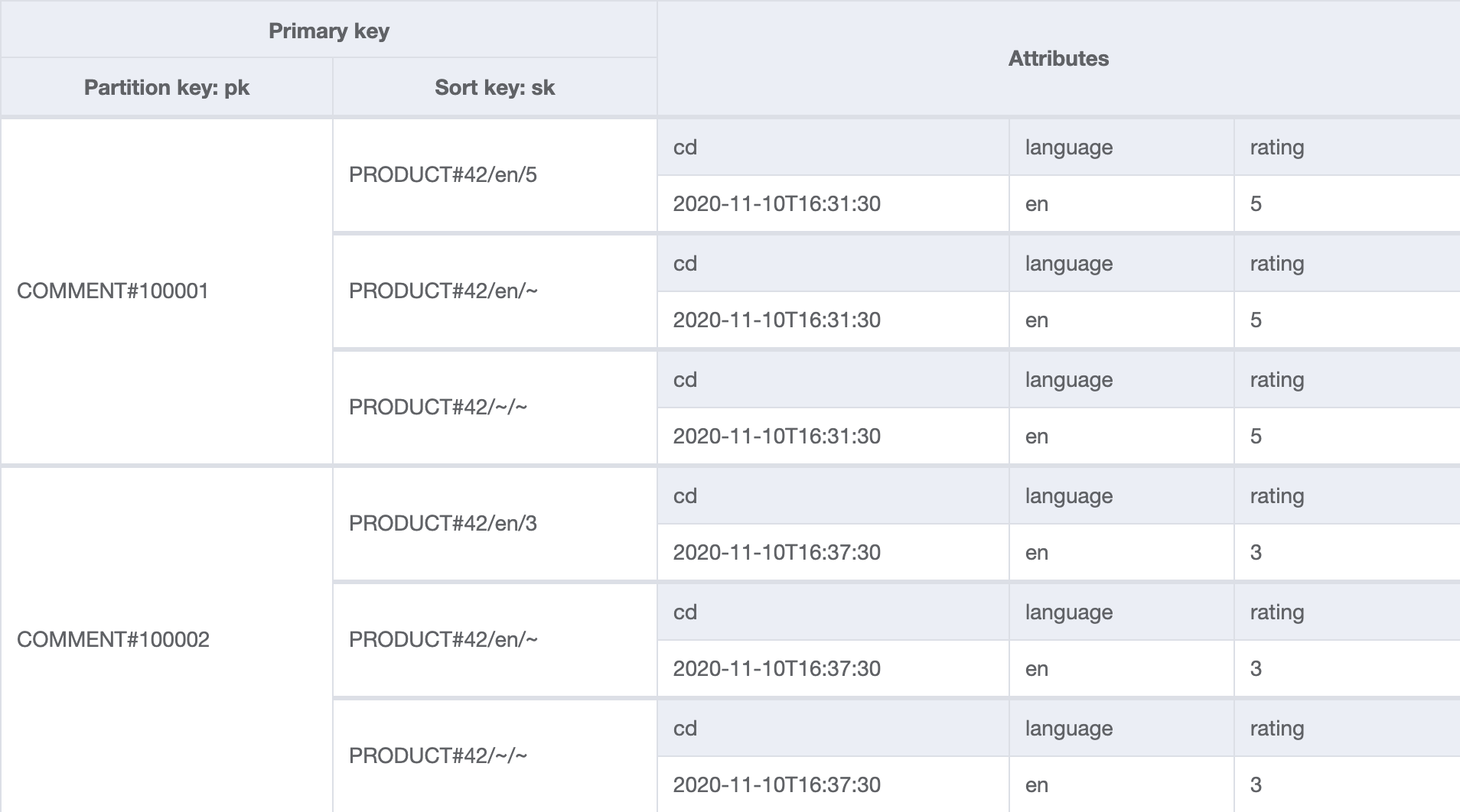
Table
The below table contains two comments for product 42. Note that there are duplicate items for each comment.
GSI
The global secondary index gsi will be used to answer the majority of the queries. Both comments exist under PRODUCT#42/~/~ (any language, any rating) and PRODUCT#42/en/~ (English, any rating). PRODUCT#42/en/5 and PRODUCT#42/en/3 contain only one comment each, as the two comments in the table are rated 5 and 3.
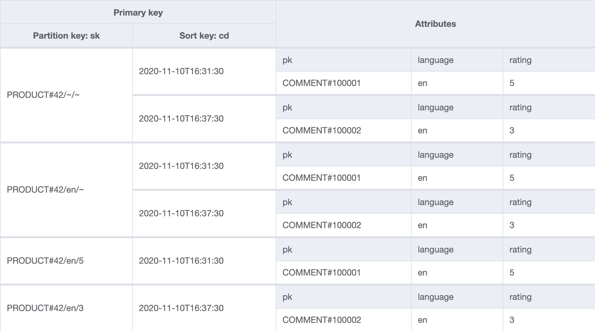
Not shown are the non-indexed attributes such as the comment text itself.
Key design
Let’s elaborate on sk. Each sk under a comment pk represents membership to a collection of comments for that product, of the criteria encoded into the key.
sk consists of a / delimited string. The first element is the type, PRODUCT# and its identifier 42. The second element is the language, such as en or ~ to denote any. The final element is the rating number, from 1 to 5.
Any combination of ratings can be specified in addition to a single selected language (or all languages).
Here are some examples:
<product>/<language>/<ratings>PRODUCT#42/~/~- any languagePRODUCT#42/en/~- English onlyPRODUCT#42/en/1- English only, with a rating of 1PRODUCT#42/en/1.2.5- English only, with a rating of 1, 2 or 5PRODUCT#42/~/1.2.5- any language, with a rating of 1, 2 or 5
It might help to think of each sk as representing an ordered set of comments. It maps neatly onto a URI such as /product/42/comments/en/1.2.3 or more likely /product/42/comments?language=en&rating=1&rating=2&rating=3.
Duplicates needed
We will assume this application will be write light and read heavy, so it is acceptable to store the same comment multiple times in order to provide inexpensive querying.
As per AP1, a user can choose to show all languages or select a single language. This can be met by double-writing the item with different sk values, once with ~ as the language element, and once with the actual language of the comment, such as en.
AP3 is more complicated as any combination of ratings can be requested. A user could select 1 to only see bad comments, or 5 to only see the good comments - or any combination of those. To achieve this, a power set is calculated to generate keys for the possible combinations. The number of items in a power set is 2 ** len(values_in_set) so in this case 2 ** len({1,2,3,4,5}) = 32 so the power set size is 32. We can remove any items from the set that do not contain the rating of the comment being posted. This brings the set size down to 16.
Ultimately, we write the comment to the table 32 times with a sk representing each combination of ratings, once for all languages and once for the actual language. A set containing multiple ratings is serialized to an ordered, .-delimited string such as 1.2.3.4.5.
You could think about each of the ratings being toggle switches that are set low or high.
00001= Rating 100010= Rating 200100= Rating 301000= Rating 410000= Rating 5
Combinations are represented as you’d expect.
10001= Rating 1 and 511111= All ratings
>>> rating_1 = 0b00001
>>> rating_5 = 0b10000
>>> bin(rating_5 | rating_1)
'0b10001'
>>> rating_5 | rating_1
17
As the combination of rating_5 and rating_1 is 17, this could be used as a more compact representation of the selected ratings, as a future optimization. Instead of PRODUCT#42/en/1.2.3.4.5, PRODUCT#42/en/31 could be stored instead.
It has the side-effect of allowing longer set values to be stored. For instance, if instead of numeric ratings we used ['Poor', 'Fair', 'Good', 'Great', 'Excellent'], the keys would be longer and we would consume more resources.
It might seem premature, but shaving bytes off repeated keys and attribute names is sometimes considered good practice as less data needs to be stored and transferred per item. The tradeoff is that this portion of the key is less readable by the human eye and therefore harder to reason about when debugging.
Queries
We should now be able to provide correct data for all of our access patterns. All queries should have ScanIndexForward set to false in order to retrieve the most recent comments first, and a Limit of 20.
AP1: Show all comments for a product, most recent first
- Query on
gsi- SK =
PRODUCT#42/~/~
- SK =
AP2: Filter by a single language
- Local language:
- Query on
gsi- SK =
PRODUCT#42/en/~
- SK =
- Query on
- All languages
- Query on
gsi- SK =
PRODUCT#42/~/~
- SK =
- Query on
AP3: Filter by any combination of ratings from 1-5
Single language
- Rating 1
- Query on
gsi- SK =
PRODUCT#42/en/1
- SK =
- Query on
- Rating 1 or 5
- Query on
gsi- SK =
PRODUCT#42/en/1.5
- SK =
- Query on
- Rating 2, 3 or 4
- Query on
gsi- SK =
PRODUCT#42/en/2.3.4
- SK =
- Query on
All languages
- Rating 5, all languages
- Query on
gsi- SK =
PRODUCT#42/~/5
- SK =
- Query on
AP4: Show a comment directly through its identifier
- Show comment
100001- Query on table
- PK =
COMMENT#100001 - Limit = 1
- PK =
- Query on table
Delete comment 100001
- Query on
table- PK =
COMMENT#100001
- PK =
Delete each value for PK/SK returned in a batch.
AP6: Paginate through comments
Run any of the above queries with Limit set to 20. Use LastEvaluatedKey returned by DynamoDB to paginate through results by passing it as ExclusiveStartKey in the next query request. Performance will be consistent, regardless of the page is being requested. This is explained in more detail in the DynamoDB docs.
Building the table
This approach works by creating redundant items with different keys. Triggers are one way of automating the creation of these duplicated items, although as we will see in the next post, they are not the only way. A DynamoDB stream should be setup on the table and connected to a Lambda function.
When a comment is created, the wildcard sk should be used, i.e. PRODUCT#42/~/~. We will call this the primary item.
The Lambda function gets invoked with a change payload when the primary item is added, updated or deleted. From the attributes language and rating, it will generate the duplicate items and add them to the table. If language and rating subsequently change, previous duplicate items will be removed before the new duplicate set is added. Upon a delete modification, all duplicate items will be removed.
An additional attribute, auto is added to the automatically created items so that the Lambda function knows to take no action in response to items that it has created in the table.
Discussion
It is expected that this simple design will perform predictably for queries. It is very simple from that perspective.
Writes are a worry, though, as we are doing a lot of duplication. There will come a point where the number of duplicates ceases to remain feasible as set cardinality increases.
2 ** 5 = 32
2 ** 6 = 64
2 ** 7 = 128
2 ** 8 = 256
...
As the number of duplicates increases, so does the number of operations and therefore cost. Changes need to the original record need to be kept in sync.
Creation of the duplicate items could partially fail. Although the Lambda will retry, it is possible that the table will be left in an inconsistent state. An hourly Lambda function could check the table, processing recent changes. Larger repair jobs implemented with Step Functions or EMR could be written to check integrity, but these may be costly to run on a large table. It is also yet more code to write.
Summary
Despite the identified caveats around excessive redundancy and storage requirements, we’ve successfully built a filtering solution without needing to use DynamoDB filters. The table is very simple to use: all access patterns can be satisfied with a single query. The read path will perform predictably.
Nothing is free of course, we have paid for this by duplicating the data and taking on the corresponding compute, write and storage costs. There is nothing wrong with duplicating data to get efficient queries. Using DynamoDB Streams and Lambda functions, duplicates are automatically maintained, without cluttering client code.
Excessive, manual duplication is still a concern, so the next post will investigate how we can reduce the storage footprint with some additional GSIs and a slightly more complicated client program.
Comments and corrections are welcome. I am working on making the diagrams exported from NoSQL Workbench more accessible.
Links
If you found this interesting, you’ll probably enjoy the following even more.